 DataMosaic

#The two lists
Every formula below runs against the same two lists. They come from an invented chain of 120 stores. ERP is the price list head office sent last night. Tills is the price list exported from the tills at ST-014 this morning. Both have two columns, SKU in A and Price in B, with headings in row 1.
| ERP: SKU | ERP: Price | Tills: SKU | Tills: Price | |
|---|---|---|---|---|
| 100231 | 4.99 | 100231 | 4.99 | |
| 100232 | 12.50 | 100232 | 11.50 | |
| 100245 | 2.79 | 100245 | 2.79 | |
| 100260 | 8.40 | 100271 | 19.99 | |
| 100271 | 19.99 | 100288 (text) | 6.25 | |
| 100288 | 6.25 | 100302 | 3.10 | |
| 100315 | 1.49 | 100315 | 1.49 | |
| 100315 | 1.39 |
Invented figures. Hidden in there: 100232 has the old price at the till, 100260 never arrived, 100302 is still on the till but no longer in the ERP, 100288 was exported as text, and 100315 is on the till twice at two prices. A good comparison finds all five and tells them apart.
#1. XLOOKUP, if your Excel has it
XLOOKUP is in Excel for Microsoft 365, Excel 2021 and Excel 2024. Its arguments, from Microsoft's page on XLOOKUP, are the value to find, where to find it, what to return, and what to show when nothing is found.
- On the ERP sheet, type
Till priceinC1. - In
C2, enter the formula below and fill it down to the last SKU.
=XLOOKUP(A2, Tills!A:A, Tills!B:B, "Missing")- Type
ResultinD1, and inD2:
=IF(C2="Missing", "Missing at till", IF(C2<>B2, "Price differs", "Matches"))XLOOKUP matches exactly by default, so there is nothing to forget. The fourth argument replaces #N/A with a word you can filter on.
Now the other direction. The ERP sheet can only show SKUs the ERP has. To find what the till has and the ERP doesn't, go to the Tills sheet and put this in C2:
=XLOOKUP(A2, ERP!A:A, ERP!B:B, "Not in ERP")Filter column C for Not in ERP. That is 100302 here, a product the ERP dropped and the till still sells. Skip this half and you never see it.
#2. VLOOKUP, in Excel 2016 and 2019
The same lookup in VLOOKUP needs two extra things: the column number to return, and FALSE at the end.
=IFNA(VLOOKUP(A2, Tills!A:B, 2, FALSE), "Missing")Never leave out FALSE. Microsoft's page on VLOOKUP says that if you don't specify it, the default is TRUE, an approximate match. On an unsorted list that returns a price from a neighbouring row with no error at all, which is worse than #N/A.
IFNA, not IFERROR. IFNA replaces only #N/A, the error that means not found. IFERROR also hides a #REF! from a broken range, so a mistake in the formula looks like a missing row.
The column number is fixed. 2 means the second column of A:B. Insert a column in the Tills sheet and the formula quietly returns the wrong one. XLOOKUP names the return column instead, which is why it is the better choice wherever you have it.
The second direction is the same formula on the Tills sheet, pointed at ERP!A:B.
#The #N/A that doesn't mean missing
Run either formula on the lists above and 100288 comes back as Missing at till, and again as Not in ERP from the other side. It is on both lists at 6.25. The tills exported that SKU as text, the ERP as a number, and an exact lookup treats "100288" and 100288 as different values. Microsoft's own page on fixing #N/A puts the wrong value type first among the causes.
To see it, put =ISTEXT(A2) next to each key on both sheets. A mix of TRUE and FALSE in one column, or TRUE on one sheet and FALSE on the other, is your answer. Then make both sides one type in a helper column, and look up the helper instead of column A:
=VALUE(TRIM(A2))TRIM removes the spaces exports like to leave at the end of a code, and VALUE turns the text into a number. When your codes have leading zeros, such as 004512, go the other way and keep them as text, so 4512 from one system becomes 004512:
=TEXT(A2, "000000")Use one six-digit format, or whatever length your codes really have, on both sheets.
#The duplicate a lookup can't see
100315 is on the till twice: once at 1.49, once at 1.39. Both XLOOKUP and VLOOKUP return the first match they find, so the ERP sheet shows 1.49 and Matches. The 1.39 that a customer may be charged never appears. XLOOKUP can search from the bottom instead, with -1 as its sixth argument, but that only swaps which row you see.
Count the keys before you trust the result. On the Tills sheet:
=COUNTIF(A:A, A2)Anything above 1 is a duplicate to look at, and only a join shows every copy side by side.
#3. Power Query: a full outer join
A Power Query merge is a join. It keeps every row from both lists, shows every match for a duplicated key, and runs again with one click when next week's files arrive. Its join kinds include Full outer, all rows from both tables, and Left anti and Right anti, the rows found on one side only, per Microsoft's merge overview.
- Click in the ERP list and choose Data › From Table/Range. Tick My table has headers and press OK.
- In the Power Query Editor, select the SKU column and set its type to Text. Then choose Home › Close & Load.
- Do the same for the Tills list.
- Select a cell in either loaded table and choose Query › Edit.
- Choose Home, the arrow next to Merge Queries, then Merge Queries as New.
- Pick the ERP query on top and the Tills query below, click SKU in each, and set Join Kind to Full Outer (all rows from both). Press OK.
- Click the expand icon on the new column, keep SKU and Price, and press OK.
Setting SKU to Text on both sides is what makes 100288 match: Microsoft notes that the columns must be the same data type, or the merge may not give correct results.
If you would rather paste one query, name the two lists as tables first (Insert › Table, then a name under Table Design), call them Erp and Tills, and paste this into Home › Advanced Editor of a blank query:
let
    Clean = (t as table) as table =>
        Table.TransformColumnTypes(
            Table.TransformColumns(t, {{"SKU", each Text.Trim(Text.From(_)), type text}}),
            {{"Price", type number}}),
    Erp = Clean(Excel.CurrentWorkbook(){[Name = "Erp"]}[Content]),
    Tills = Clean(Excel.CurrentWorkbook(){[Name = "Tills"]}[Content]),
    Merged = Table.NestedJoin(Erp, {"SKU"}, Tills, {"SKU"}, "Till", JoinKind.FullOuter),
    Expanded = Table.ExpandTableColumn(Merged, "Till", {"SKU", "Price"}, {"Till SKU", "Till price"}),
    WithKey = Table.AddColumn(Expanded, "Key",
        each if [SKU] = null then [Till SKU] else [SKU], type text),
    WithResult = Table.AddColumn(WithKey, "Result",
        each if [Till SKU] = null then "Missing at till"
        else if [SKU] = null then "Not in ERP"
        else if [Price] <> [Till price] then "Price differs"
        else "Matches", type text),
    Sorted = Table.Sort(WithResult, {{"Key", Order.Ascending}})
in
    Sorted
Choose Home › Close & Load, and the result lands on its own sheet. When the next files come in, paste them over the old lists and choose Data › Refresh All.
#The worked example
Here is what each method says about the eight till rows and seven ERP rows above:
| SKU | ERP | Till | XLOOKUP, both ways | Power Query, full outer |
|---|---|---|---|---|
| 100231 | 4.99 | 4.99 | Matches | Matches |
| 100232 | 12.50 | 11.50 | Price differs | Price differs |
| 100245 | 2.79 | 2.79 | Matches | Matches |
| 100260 | 8.40 | none | Missing at till | Missing at till |
| 100271 | 19.99 | 19.99 | Matches | Matches |
| 100288 | 6.25 | 6.25 | Missing at till, and Not in ERP | Matches |
| 100302 | none | 3.10 | Not in ERP | Not in ERP |
| 100315 | 1.49 | 1.49 | Matches | Matches |
| 100315 | 1.49 | 1.39 | not shown | Price differs |
Invented figures. The lookups get two rows wrong: they report 100288 missing on both sides when it matches, and they never show the second 100315. The merge gets all nine right because both keys were made text first and a join keeps every match. Each real result sends you somewhere different: 100232 and 100315 to the price batch ST-014 should have loaded, 100260 to the file that should have carried it, 100302 to whoever retires products on the tills.
#Which one to use
- One list, once, Excel 365, 2021 or 2024: XLOOKUP, both ways, with an ISTEXT glance at the keys.
- Excel 2016 or 2019, or a workbook others open in old versions: VLOOKUP with FALSE, inside IFNA.
- A key that can repeat, a key made of two columns, or the same comparison every week: Power Query. Select both columns with Ctrl in the merge dialog for a two-column key, such as store and SKU, rather than building a helper column.
- Two whole sheets, row by row: see how to compare two Excel files. For files too large to open, see comparing two CSV files.
#Where doing it by hand runs out
The price file in this post is one store, one night. A chain of 120 stores has 120 till lists every morning, and the merge only runs when someone exports the files, pastes them in and presses Refresh. It finds 100232 at the old price. It doesn't say whether the batch failed to send, failed to load, or was overwritten, and it doesn't send it again.
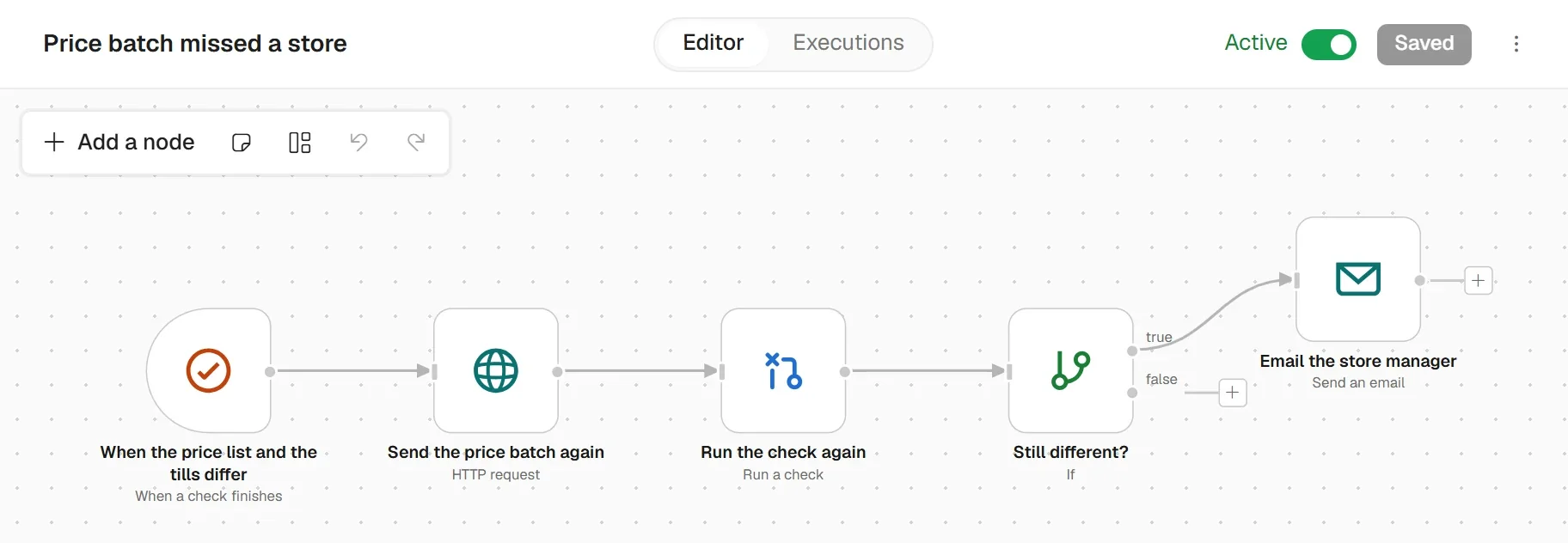
DataMosaic does this comparison as a check. It reads the systems themselves, or their CSV and Excel exports when there is no connection yet, lines the sources up on shared keys, and shows matched, differing and missing rows. Normalising makes two systems read the same way before anything is compared, so S014 and 014, or text and number, stop being a difference. Rules decide when a run fails, and a schedule runs the check before anyone arrives. A check only reads. Mosaic changes a system only through a workflow you build, such as sending the price batch again and running the check once more.
#Questions people ask
#How do I use VLOOKUP to compare two columns and find missing values?
Look up each value of the first column in the second with =IFNA(VLOOKUP(A2, Sheet2!A:A, 1, FALSE), "Missing"). Every Missing is a value the second column lacks. Repeat from the second column into the first to find what the first one lacks.
#Why does VLOOKUP return #N/A when the value is there?
Usually because one side is a number and the other is the same digits stored as text, or one has a trailing space. Check with ISTEXT, then convert both sides with VALUE(TRIM(A2)), or with TEXT if the codes have leading zeros.
#Is XLOOKUP better than VLOOKUP for comparing lists?
Where you have it, yes: it matches exactly by default, names the return column instead of counting to it, and takes a not-found value without IFNA. It is in Excel for Microsoft 365, 2021 and 2024.
#How do I compare two lists in Excel when there are duplicates?
A lookup returns only the first match, so count each key with COUNTIF first. To see every copy next to its match, merge the two lists in Power Query with a full outer join.
#Can Power Query compare two columns?
Yes. Merge the two tables on the column, choose Full Outer to see everything, or Left Anti or Right Anti to list only the rows missing from the other side.